MRI
Contents
What follows is an explanation of how the seemingly mysterious, quantum-mechanical, magnetic properties of atomic nuclei enable the generation of non-invasive images of the inside of the body. Here we avoid all of the underlying maths (if you are interested in that aspect, there is a great deal of technical literature about the topic of magnetic resonance).
We begin with an overview of the magnetic resonance branch called nuclear magnetic resonance (NMR) spectroscopy. This is a useful first step, as it will help to illustrate many of the underlying and enabling scientific principles of MRI too. Once we have outlined conventional NMR spectroscopy principles, the step to MRI is broadly about how to encode spatial information (that is: where the various signals are coming from) to generate images for medical diagnosis. Finally, magnetic resonance is a rapidly expanding field of research and applications. To keep this page future proof, at least for a little while, we also discuss some more recent developments in magnetic resonance.
The basics: nuclear magnetic resonance (NMR) spectroscopy
Nuclear magnetic moments / nuclear spin
Magnetic resonance methods exploit the microscopic behaviour of the magnetic moments of atomic nuclei. These magnetic moments arise because of the intrinsic angular momentum (quantity of rotation) of the positively charged atomic nuclei, causing them to have a permanent magnetism. This form of microscopic angular momentum is known as spin (the spin of an individual sub-atomic particle is quantised to I = ± ½) . Very nearly all chemical elements in the periodic table of the elements have at least one isotope with non-zero spin and can be used, in principle, to obtain NMR spectra. For an atomic nucleus to have non-zero spin, the nucleus must either have an odd mass number (yielding half-integer spin values; for example 1H or 13C) or an even mass number resulting from odd numbers of both neutrons and protons (yielding integer spin values; for example 2D or 14N). Only atomic nuclei with non-zero spin can produce magnetic resonance effects. Unfortunately, some chemically and biologically important chemical elements have majority isotopes with zero spin (for example carbon: 99 % of naturally occurring carbon isotopes are 12C, made up from six neutrons and six protons, yielding zero spin; only 1 % of carbon atoms are of the 13C variety, with spin I = ½). By the way, we only talk about stable, non-radioactive isotopes (MRI is a non-invasive method)!
The abstract concept of spin and magnetic moment in the microscopic world (in sub-atomic particles such as protons, electrons, neutrons and photons) has no analogy in the macroscopic world. That, however, is the world in which we (as macroscopic bodies) live and what we can intuitively understand from our own experiences of the macroscopic world around us. It is probably best just to accept the seemingly bizarre behaviours and properties of the microscopic world, ruled by quantum mechanics, without trying to find an analogous picture in the macroscopic world – this would be bound to be wrong at some level. Some theoreticians even go as far as stating that ‘spin’ may be nothing else but the expression of a weird and wonderful mathematical property. No wonder that about 100 years ago, when the first experimental discoveries of spin were made and could no longer be ignored or dismissed, classical physics did their very best to deny the presence of anything that comes in multiples of ½ (such as spin) for the longest possible time!
Spin precession / Larmor frequency
Spin and magnetic moment of an atomic nucleus can be represented by a vector. Vectors are quantities that have both a magnitude and a direction; this is relevant in our description of their behaviour when placed in an external, strong and homogeneous magnetic field, B0. External magnetic fields used in NMR spectroscopy or clinical MRI (see below) can also be represented by a vector: B0. In NMR spectroscopy this vector usually has its principal (main) direction arranged vertically, B0 in MRI is arranged horizontally.
Figure 1 illustrates the effect of the presence of a strong external magnetic field B0 on a magnetisation vector m.
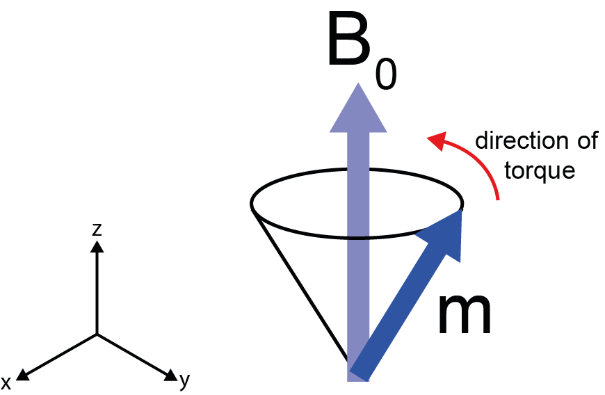
The magnetic field exerts a torque on the magnetic moment, causing it to move in a cone around the main direction of the field. This type of motion is called precession and it does have parallels in the macroscopic world. Think of a child’s spinning top. If the top is spun on a vertical axis, its motion is stable. If the axis is tilted, the force of gravity pulls it to the ground. However, if the top has enough angular momentum (if it is spinning fast enough), it will not fall over but instead will precess in a circle around its axis of rotation.
The magnetic moment vector precesses around the B0 field principal direction at a frequency that is characteristic for each isotope and is proportional to the strength of the B0 field (thus we can start to see how frequency may be be used as a fingerprint to identify different nuclei/isotopes within a sample/body). This characteristic precession frequency is called Larmor frequency (after the Irish physicist and mathematician Sir Joseph Larmor). For example, in a B0 field of strength such that the 1H (hydrogen, I(1H) = 1/2) Larmor frequency is 400 MHz, the 13C (carbon, I(13C) = 1/2) Larmor frequency will be 100 MHz. The order of magnitude of these frequencies lies within the radio wave carrier band of the electromagnetic spectrum.
From a single spin to a macroscopic sample
An NMR spectroscopy sample will not be just a single spin (as we have considered so far) but a sample is made up from a very large number of identical spins or groups of spins (called an ensemble), all ‘packed/contained’ in a very large number of identical molecules. That is what one would normally call a chemically pure sample.
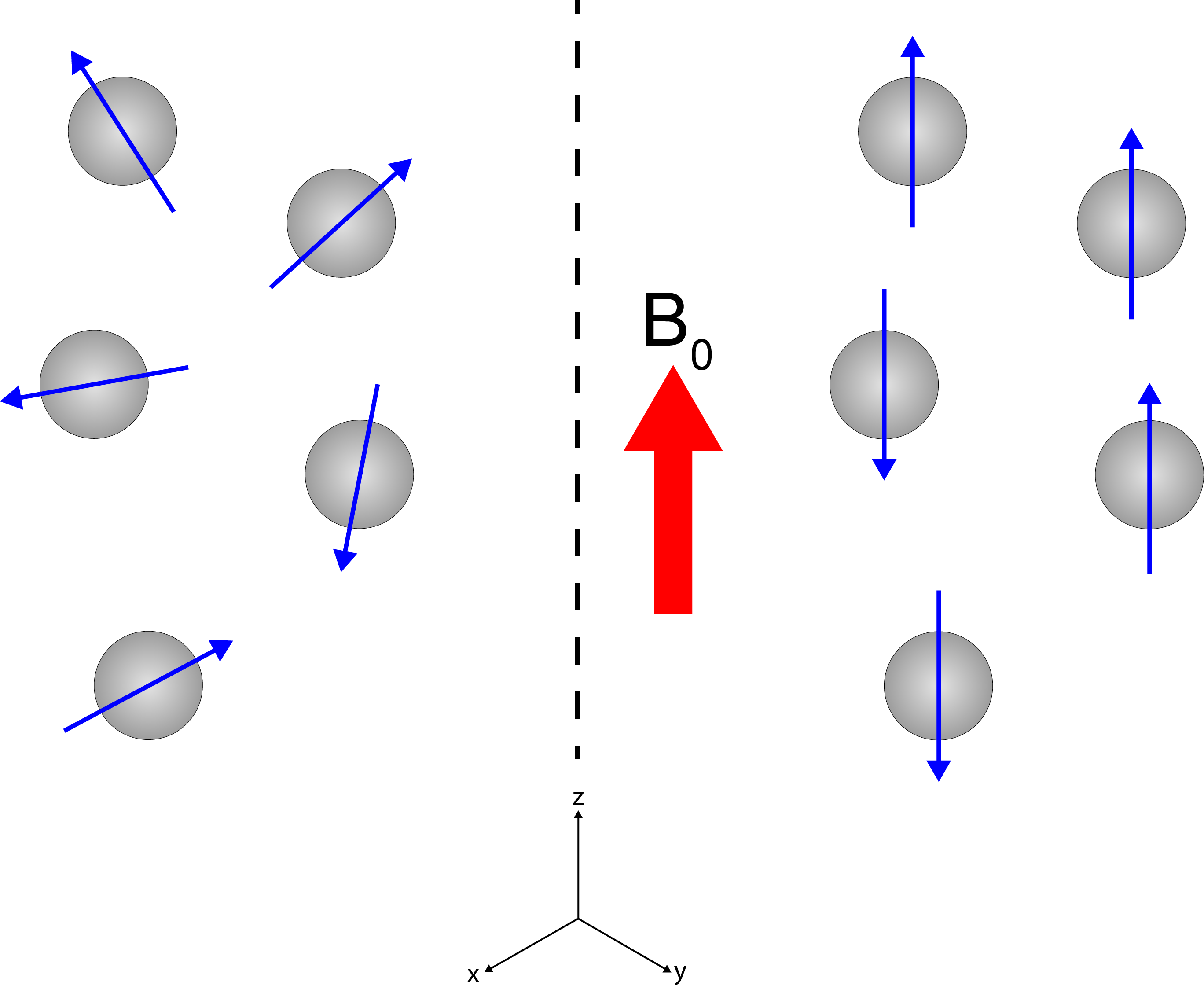
The left part of Figure 2 shows that in the absence of the B0 field, the nuclear magnetic moments / spins are randomly oriented and move randomly. The right part of Figure 2 illustrates that when the sample is placed in the strong magnetic field B0, averaged over time there is a small surplus of orientation / alignment with the B0 main direction. This small surplus, again can be represented as a vector (similar to Figure 1) but now represents the macroscopic net nuclear magnetisation of the whole sample. It is still a tiny surplus because not much is gained energetically from alignment with the external magnetic field relative to the thermal energy at ambient conditions (this is one of several reasons why it takes considerable amounts of time to accumulate NMR spectra – or MRI scans: there is not much surplus to ‘harvest’ for spectroscopy or imaging).
From a macroscopic sample to a (typical) NMR spectrum
So far, we cannot see why NMR spectroscopy is one of the most important analytical spectroscopy tools in contemporary chemistry, biochemistry, materials science and pharmacology laboratories. We have not yet explained what makes these tiny nuclear magnetic moments such a great source of information about materials and samples and their molecular structures.
A look at a cartoon of the 1H NMR spectrum of ethanol, EtOH (Figure 3), helps to explain this role.
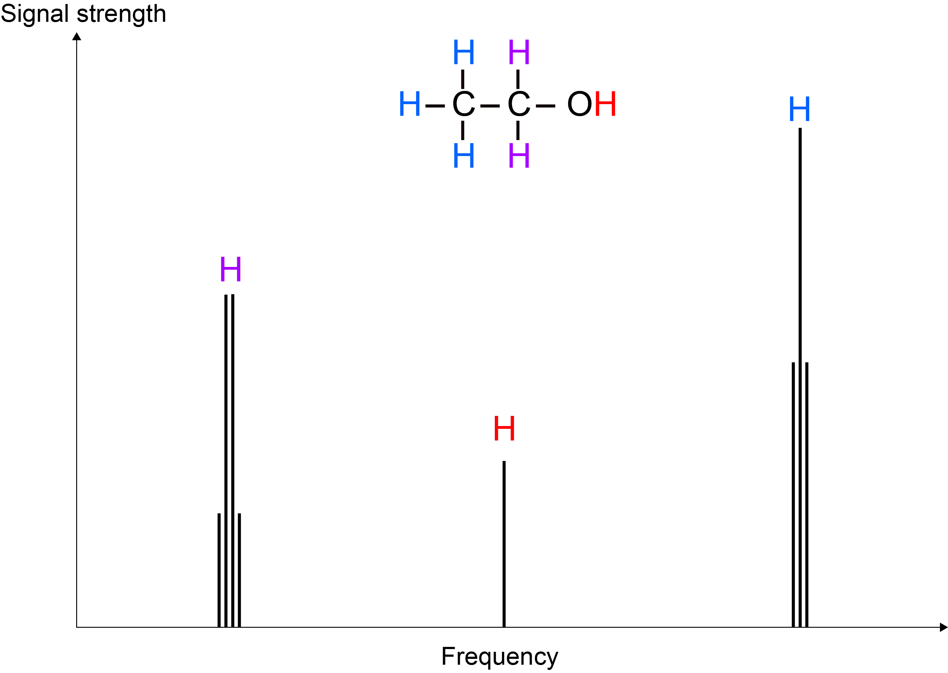
The EtOH molecule features three slightly different types of hydrogen chemical environment: CH3, CH2 and OH. This difference gives rise to ever so slightly different Larmor frequencies for the corresponding three types of 1H nuclei, yielding three different peaks in a frequency spectrum plot. This difference in frequencies arises because each of the three types of 1H environments ‘feels’ B0 slightly differently – this effect is called chemical shift (because it traces chemical differences of sites in molecules) and is a very small effect, compared with the effect of the large B0 field. If B0 induces a Larmor frequency of, say 400 MHz, then the whole range of chemical shifts for all types of reasonably common 1H chemical situations amounts to a range of approximately 4 kHz. The relative intensity of the three peaks in the 1H NMR spectrum of EtOH (3 : 2 : 1) reflects the relative abundance of the three types of H atom sites in the molecule.
A closer look at the different peaks in the 1H NMR spectrum of EtOH reveals fine structure of the peaks. These splitting patterns arise from 1H spins not only sensing the large B0 field but also the presence of the various other (tiny) magnetic moments of the other nearby 1H spins. In NMR spectroscopy of liquids, this ‘indirect dipolar coupling’ effect between 1H spins within a molecule is of the order of 1 to 100 Hz.
In short, NMR spectroscopy is a highly informative method to characterise structure and connectivity of molecules and materials at an atomic-resolution scale, without destroying the sample.
Samples and (typical) NMR spectrometers
Not destroying the sample by recording NMR spectra is an important practical consideration in everyday laboratory practice. As a consequence of the only tiny magnetisation surplus to exploit for the creation of NMR spectra, a much larger amount of sample is needed to obtain NMR spectra than is required for other analytical methods, such as mass spectrometry or vibrational spectroscopy.
Figure 4 shows typical sample containers for NMR spectroscopy of liquids and powdered solids.
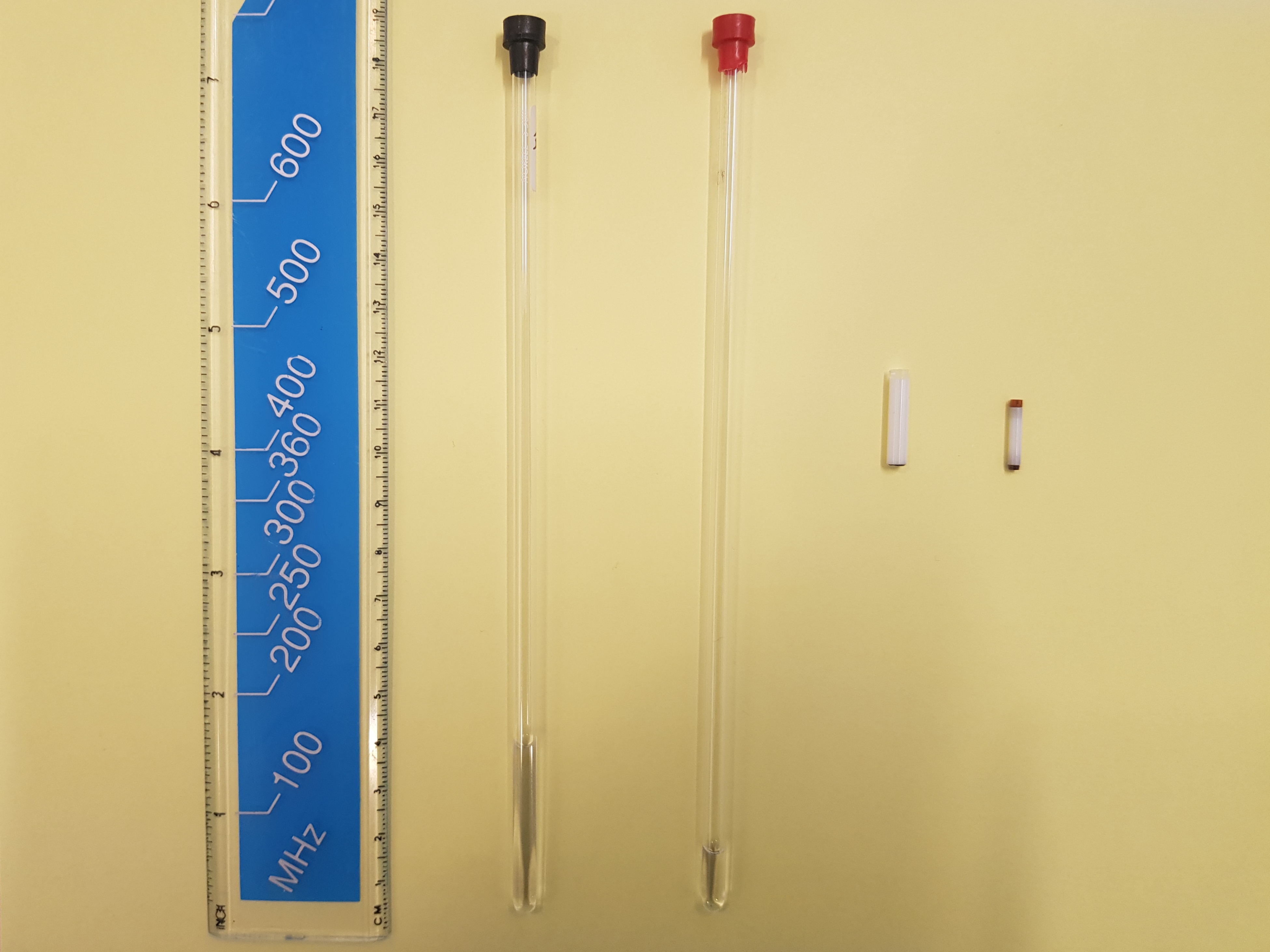
These samples are completely homogeneous. That is necessary to reveal all the fine details of molecular-structure information in NMR spectra (Figure 3). An anecdotal remark: the dimensions of the (very expensive) ceramic solid-state NMR spectroscopy sample holders (Figure 4) are such that many solid-state NMR laboratories have good collections of dental tools that are normally used for root canal treatment for handling powdered samples.
Figure 5 shows a typical NMR spectroscopy laboratory with a number of spectrometers.
The large ‘pots’ contain the magnets at their centre (the magnet is much smaller than the container): the magnet is a solenoid coil made from superconducting wires. These provide the strongest, most stable and homogeneous magnetic fields. Superconducting magnets need permanent cooling by liquid He, plenty of thermal insulation around that cooling bath, and including another cooling bath (liquid nitrogen) around that. In addition, the spectrometer needs a computer console to control its operation, and some radiofrequency equipment (transmitters, frequency filters, amplifiers, etc.) to manipulate the spin / magnetic moments with. Superconducting magnets certainly look big and mighty but, in fact are quite fragile creatures and are easily perturbed (or destroyed). Figure 6 gives a schematic overview of the set-up of a typical NMR spectrometer. The samples are placed in a probe in the core region of the magnetic field and samples are lifted in/out either by levitation or by removing the probe that holds the sample in the magnet centre. Sample changes may be automated for screening of large numbers of routine samples in some analytical applications of NMR spectroscopy.
How to manipulate the magnetisation vector to obtain spectra
Now we need to answer the question: how did we actually produce the 1H NMR ‘spectrum’ of EtOH? The answer is contained in the acronym NMR where R stand for ‘resonance’. We irradiate the precessing nuclear magnetic moments with a short (microseconds), sharp electromagnetic pulse of the ‘right’ frequency, that is the frequency of the precession (Larmor frequency; the ‘right’ frequencies are in the radiofrequency range for most areas of NMR spectroscopy). This resonance flips the magnetisation vector from its equilibrium alignment with the B0 field in the z-direction into the x,y-plane (Figure 7). This is sometimes called a 90° pulse. In the x,y-plane we observe what happens over time, after the short, sharp pulse is switched off. This response to the disturbance by the radiofrequency pulse produces the spectral signatures as shown in Figure 3.
In more detail, the perturbed magnetisation vector continues to precess around the main magnetic field B0. This is akin to a rotating magnet – and just like a wind turbine, this will generate an electric current in a nearby wire. The recording of the NMR spectra occurs as the recording of this oscillating induced electric current over time. The oscillation is a superposition of the characteristic Larmor frequencies for the different chemical environments. Both time and frequency domains, obviously, contain identical information, but for spectroscopy applications it is often preferable to display information as a function of frequency (such as the cartoon of a 1H NMR spectrum of EtOH displayed in Figure 3; see above). It is easy to toggle between these two domains, the (widely used in engineering and sciences) mathematical operation Fourier transformation toggles between the time/frequency domains.
What the magnetisation vector does after the disturbance by the pulse: relaxation
After the pulse is turned off (Figure 7), the magnetisation vector in the x,y-plane loses its coherent behaviour, it dephases. The decay of signal over time is the effect that is measured when NMR spectra are recorded. In addition to this decay of the signal in the x,y-plane, over time also the original equilibrium net magnetisation aligned with the B0 direction along the z-axis rebuilds (Figure 8).
The relaxation timescale / rate constant for decay of magnetisation in the x,y-plane is called T2 relaxation. The observed signal is called the free induction decay (FID). The relaxation timescale / rate constant for return to equilibrium along the B0 field in the z-direction is called T1 relaxation. These two relaxation processes, following the disturbance by a radiofrequency pulse, are two very different types of relaxation. Both of them depend strongly on the state of matter and tend to be very different for different materials and/or different isotopes. This is summarised in Figure 9.
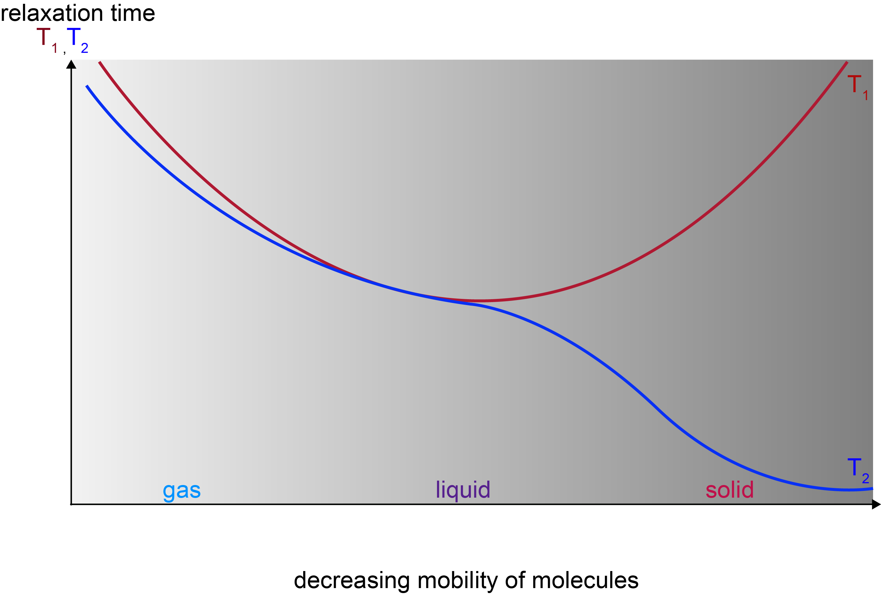
For small molecules in liquids a typical time scale for both T1 and T2 is of the order of a few seconds; for a very rigid material T1 timescales can be of the order of minutes to hours, while T2 timescales may be of the order of fractions of a second. These ‘NMR timescales’ are very slow in comparison with timescales in other spectroscopic methods.
The nuclear magnetic moments are well isolated from the outside world and all relaxation in magnetic resonance is so-called stimulated relaxation. Stimulated relaxation relies on some driving / kicking force to trigger relaxation, rather than relaxation being a spontaneous process (stimulated relaxation also underlies the working principles of lasers). Such relaxation help in magnetic resonance comes from molecular motion with the right kind of frequency and amplitude (hence the strong T1/T2 dependencies on the mobility of molecules/materials/tissues). Another mechanism for aiding relaxation comes from interactions of the nuclear magnetic moments with other magnetic moments. The most important of these interactions is with the magnetic moment of electrons. The large magnetic moment of unpaired electrons in paramagnetic molecules is the reason why such paramagnetic compounds serve as contrast agents in MRI (see below).
Measuring T1 relaxation times
T1 relaxation is commonly measured by a technique named inversion recovery (Figure 10). T1 relaxation concerns the magnetisation vector m and its alignment with the z-direction / main magnetic field B0. Accordingly, an experiment to measure T1 relaxation times needs to monitor the behaviour over time in that direction.
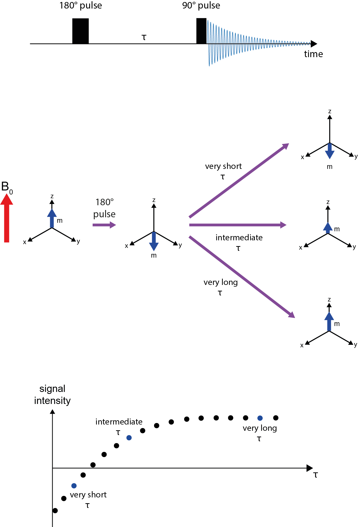
Using a 180° radiofrequency pulse, the magnetisation vector is inverted, to point in -z-direction (now anti-parallel to the main magnetic field). A time period, τ, is waited before a 90° radiofrequency pulse is used to flip the magnetisation vector at that point in time into the x,y-plane, the signal (see Figure 8) is recorded and the amplitude of the signal determined. The amplitude of the recorded signal depends on the duration of the waiting period τ. If τ was very short, not much T1 relaxation will have occurred and an intense, negative signal is observed. If τ was very long, the magnetisation will have been completely re-established along the z-direction and an intense, positive signal is recorded. Intermediate durations of τ yield intermediate intensities of positive or negative signals after read-out, including one particular value of τ for which a zero-signal is obtained. An array of experiments is run with a set of different durations of τ delays. From the resulting graph, plotting signal intensity against τ, the T1 relaxation times are calculated.
Measuring T2 relaxation times
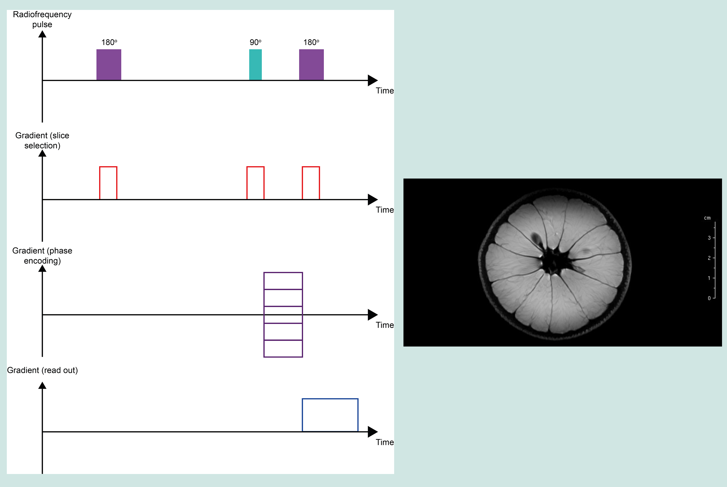
T2 relaxation times are measured by a so-called spin-echo pulse sequence. T2 relaxation concerns magnetisation decay in the x,y-plane and thus, the spin-echo experiment observes echo formation in the x,y-plane (Figure 11).
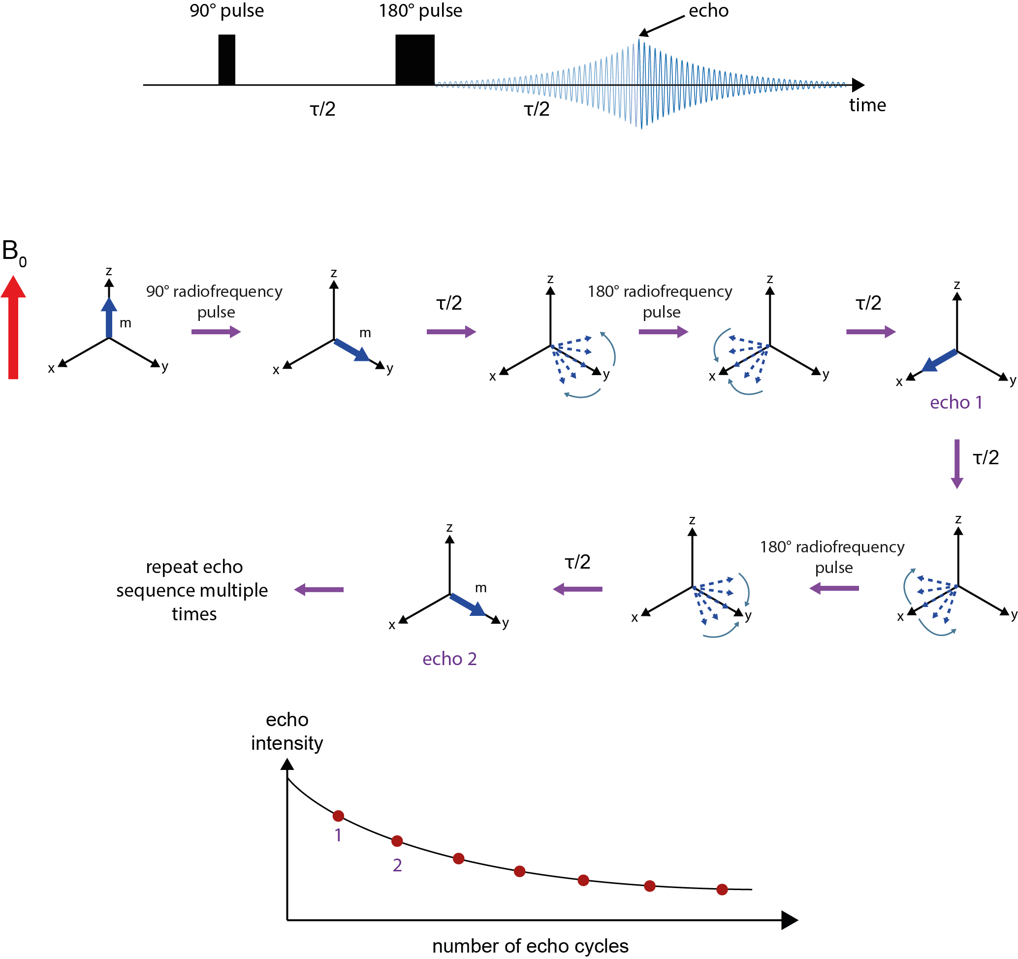
After equilibrium magnetisation is established in the z-direction, a 90° pulse flips the magnetisation vector into the x,y-plane, followed by a waiting period τ/2. During this period, genuine T2 relaxation takes place, but also additional decaying/dephasing of the signal caused by imperfections of the sample and very slight inhomogeneities of the B0 field over the sample volume. A 180° pulse, applied after waiting for period τ/2, reverses the effects of these fixed apparent (called T2*) relaxation mechanisms by reverting the sense of precession. After waiting another period of τ/2, an ‘echo’ forms where all vectors are aligned and the magnitude of that vector at this moment in time reflects the true T2 relaxation effects over the delay period (at this point in time the decaying/dephasing of the signal caused by imperfections of the sample and very slight inhomogeneities of the B0 field is eliminated). At this point in time, τ, the amplitude of the echo is recorded. From this point the remaining signal again starts to decay through dephasing caused by imperfections of the sample and very slight inhomogeneities of the B0 field. The application of 180° radiofrequency pulses can be repeated at further periods of τ/2 to generate further echoes. These observations can be repeated until the echo amplitude reaches zero. A graph where echo amplitudes are plotted against time / number of echo cycles permits calculation of the T2 relaxation time (an estimate of T2* can be obtained from the exponential decay of an ordinary time-domain signal, without the application of the 180° radiofrequency pulses (see Figure 7)).
Consider a sample made up from different components, for example a body with all its different tissues and organs. These components will each by characterised by different T1, T2 and T2* decay times dependent upon their chemical environment and tissue mobility (see Figure 9). If we take a snapshot by recording the 1H magnetic resonance signal of all these different 1H environments, the signal strength for each environment will be weighted by its T1, T2 and T2* decay characteristics. These intensity data can be used to create ‘images’ – this is the basic driving idea of magnetic resonance imaging, MRI.
Magnetic resonance imaging, MRI
There will be some differences between NMR spectroscopy and clinical MRI investigations. First of all, think of a human being as the sample for MRI. Other than in NMR spectroscopy, a body is not a homogeneous sample and it is much bigger than typical spectroscopy samples.
This immediately explains the following two considerations; i) there are different design criteria for the magnets used in MRI scanners; and ii) the valuable spectroscopic, high-resolution parameters (chemical shifts, fine structure in spectral peaks by coupling interactions between nuclear magnetic spins) may not be of much use or interest when aiming to create three-dimensional images. Instead, more global parameters (such as relaxation characteristics T1 and/or T2, and/or T2*) are a more suitable base for imaging purposes, provided methods can be found to encode spatial information in magnetic resonance experiments.
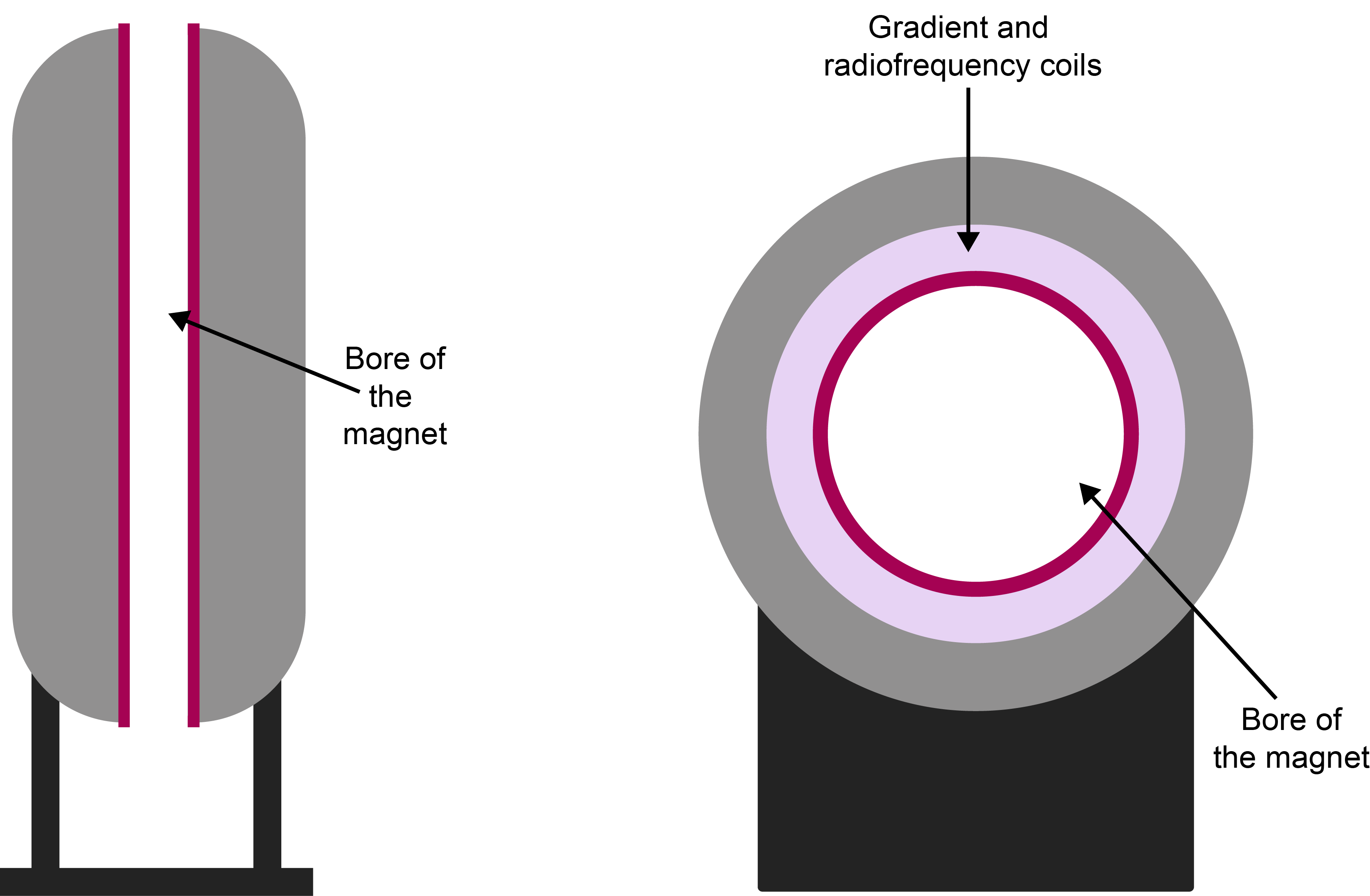
Figure 12 contrasts the different magnet designs in NMR spectroscopy and MRI. In clinical MRI, the bore of the magnet is oriented horizontally (vertically in NMR spectroscopy) and has to be wide enough to accommodate a human body when lying down in supine position.
Placing a body in such a horizontal homogeneous magnetic field and recording a 1H NMR spectrum of the body would be a rather useless exercise. The inhomogeneous body with its myriad of different compounds and tissues would just give a very broad hump of a 1H NMR spectra of all these components superimposed on each other. There would be no spatial information and no contrast. At this point, we abandon the spectroscopy aspects of magnetic resonance. MRI typically makes no use of these high-resolution spectroscopic signatures. Instead, MRI tends to focus on the 1H magnetic resonance signal of ubiquitous water molecules, and uses differing relaxation characteristics of the different chemical/biological environments to provide contrast
How spatial encoding works in MRI
In an MRI scan, the image reconstruction methods used must be able to localise individual signals in three-dimensional space. This is achieved by inducing a known varying magnetic field across a particular dimension on the sample. This is known as applying a magnetic field gradient (Figure 13) and is simply induced by passing a current through a coil (known as a gradient coil).
As the magnetic field varies across space (for example, low to high from left to right; Figure 13), the 1H resonance frequency will vary too (low to high from left to right); we have thus ‘encoded’ the signal with spatial information. The resulting signal is a superposition of all of these frequencies. All the underlying frequencies can be identified and if we measure a high frequency response, this must have come from the right hand side of the sample. Gradient coils are not powered all the time, but are switched on and off due to the heat they produce (through resistance to the current).
By matching the applied radiofrequency pulse to the 1H resonance frequencies of protons at a particular position, a section or slice of the sample / body can be ‘selected’ to be imaged. Protons in the vicinity but with different 1H resonance frequencies will not be excited by such a selective pulse and thus will not contribute to the read-out data.
This slice-selection gradient is applied in the z-direction (Figure 13) at the same time as the radiofrequency pulse. In theory, an extremely narrow-banded radiofrequency pulse will select an extremely thin slice of the scanned object / body. In practice, the pulse contains a range of frequencies known as the transmission bandwidth. The thickness of the selected slice can be changed by varying the bandwidth. By increasing the thickness, the amount of read-out signal is increased – as there are more protons in a thicker slice, and this extra signal can speed up image acquisition time. However, this decreases image resolution. In practice, a compromise has to be found between required image resolution and feasible scanning times.
So now we have perturbed a thin slab of nuclei in our sample/patient using the aptly named ‘slice selection gradient’ in the z-direction. Gradients in the x- and y- directions are then used for further localisation within said slice/slab. The NMR signals arriving at the detector originate from the whole selected slice and are a superposition of frequencies. To localise a signal within the slice region, a technique called back projection is used (Figure 14). Back projection involves measuring the frequency spectrum with multiple different gradient directions applied across the sample sequentially. Each new perturbation must start from the equilibrium position of the magnetisation vector, and the number of different directions of the gradient determines the resolution of the final image. So, assuming T1 of 1H in water molecules is 1s and we want a 256 × 256 image, this would take about 12.5 minutes to acquire (3 × T1 × number of gradients). Comparing the resulting spectra we are able to reconstruct the spatial location/origin of a particular signal. This form of reverse-engineering of read-out data in MRI is reminiscent of similar analysis methods used to reconstruct three-dimensional images from CT scans.
More modern approaches to spatial encoding utilise the same three gradients. However, alongside encoding with frequency, one gradient is used to encode phase coherence, making use of the fact that the signals used not only have a frequency and intensity but also a phase.
A slice-selection gradient can in fact be applied in any direction, using the three gradient coils. This gives freedom to image an object in any plane chosen. Standard geometries are the axial, sagittal, and coronal planes (Figure 15) as is also common in the inspection of three-dimensional CT images. Oblique planes, in addition to coronal, sagittal and axial planes, can also be useful when having to characterise asymmetric three-dimensional features.
Similar to CT scans, MRI data is stored in three-dimensional voxel arrangements, allowing a faithful representation of the scanned object. However, in CT scans, images are generally acquired in the axial plane; this axial data set is then used to reconstruct images in the other planes (usually the sagittal and coronal planes). In contrast, MRI data sets can be acquired in any plane, depending on the choice of gradients used in the scan.
Gradient Echo Sequences in MRI
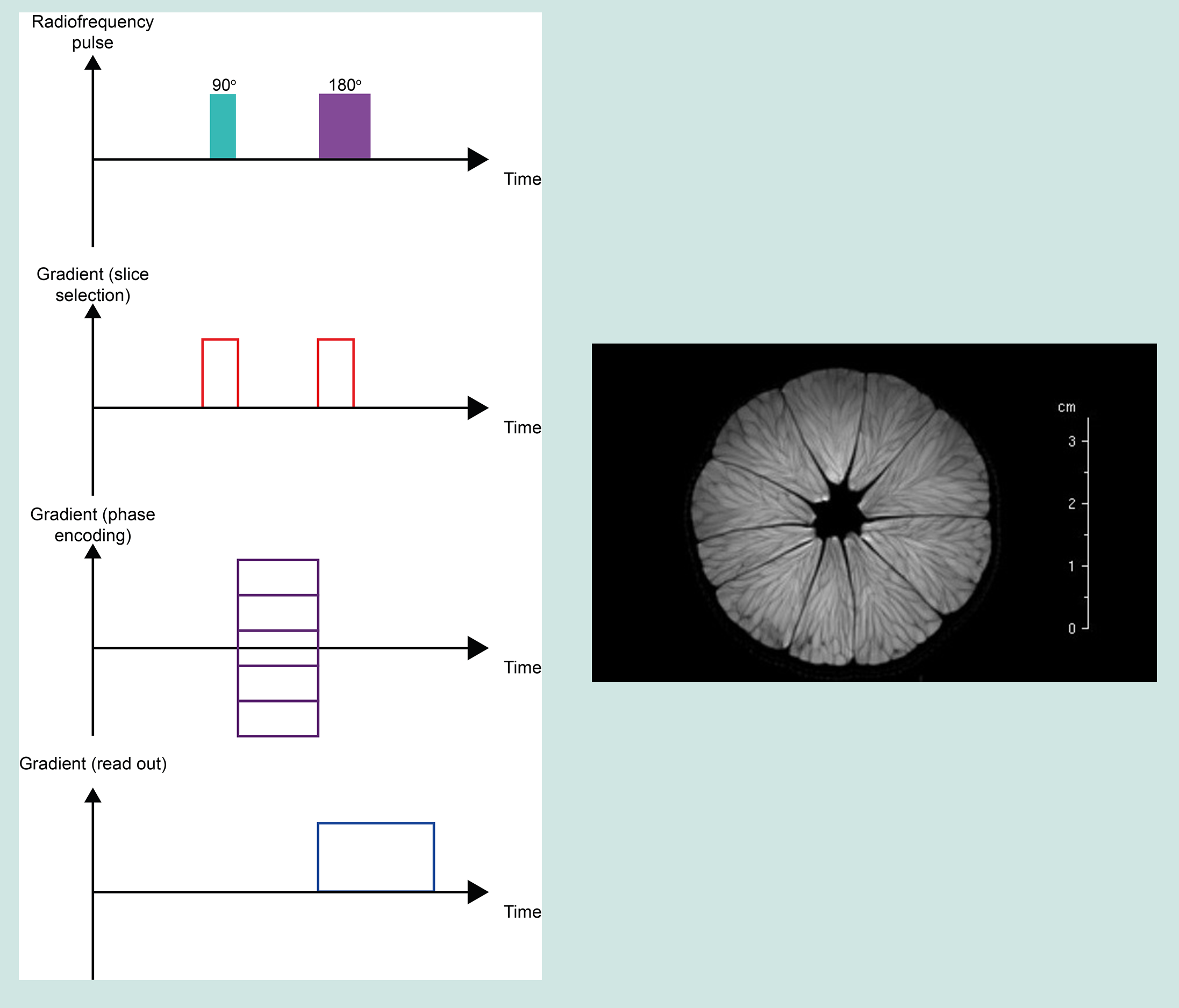
Spin-echo sequences that are used to measure T2 relaxation rates in NMR spectroscopy (see above, Figure 11) use a pair of radiofrequency pulses, a 90° excitation pulse and a 180° refocusing pulse. The gradient echo sequence used in MRI, consists of a single radiofrequency excitation pulse in conjunction with a gradient reversal that replaces the 180° pulse. The gradient-echo sequence differs from the spin-echo sequence in yet another way: the flip angle of the initial radiofrequency pulse is usually less than 90° to decrease the amount of magnetisation tipped into the x,y-plane such that there is a faster recovery of z-magnetisation and thus the total imaging time is shortened (for example, using a 30° radiofrequency pulse instead of a 90° pulse approximately halves the scanning time). The gradient echo is generated by a magnetic field gradient (Figure 16). One gradient is used for slice selection as usual, one for measurement, and one to manipulate the phases of spins.
Gradient-echo sequences generally have faster imaging times in comparison to spin-echo sequences due to the low initial flip angle. However, the gain in speed of the experiment may be counteracted by some artefacts in the resulting data set. The absence of a refocusing radiofrequency pulse means that effects of magnetic field inhomogeneities on the spin dynamics are not removed (as is done in a spin-echo experiment). This is important for imaging of the oral cavity, where inhomogeneities caused by magnetic-susceptibility differences between air and water play a role. These experimental imperfections can result in accumulation of phase errors, leading to positioning errors in the phase-encoding direction.
Effects providing contrast in MRI
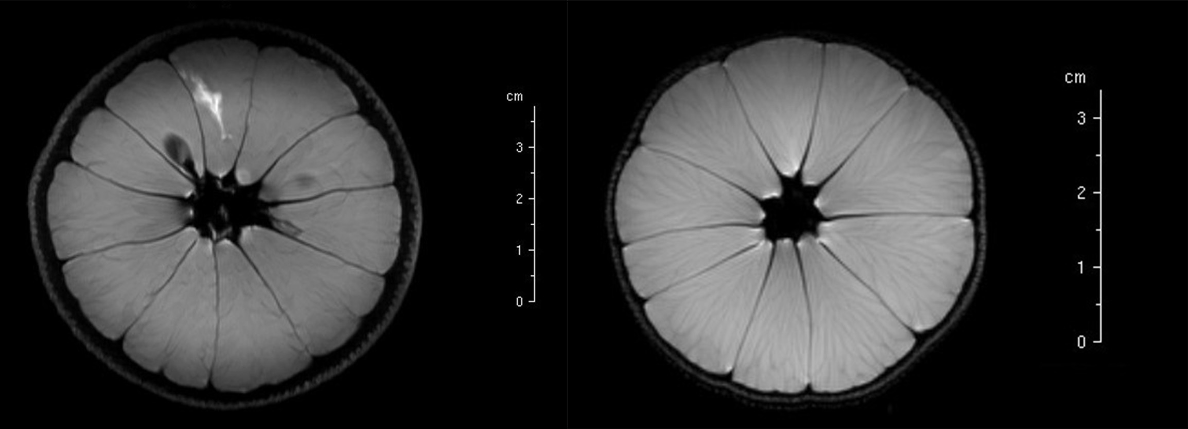
MRI images are typically depicted in shades of grey, varying from black to white. The specific shade of grey of a scanned structure is determined by signal intensity in a specific region. Image contrast originates from a combination of the T1 and T2 relaxation times, and the density of spins of the various substances / structures / tissues in the scanned object (Figure 17).
For example, in the specific case of MRI scans of the brain, tissues have minor differences in structure and texture, still leading to a range of different T1 and T2 relaxation times for different regions in the brain (Table 1). Some values are characteristic, others display overlap with characteristics of other tissues.
Table 1 Typical T1 and T2 relaxation times of tissues in the brain
| Tissue type | T1 (s) | T2 (s) |
|---|---|---|
| cerebrospinal fluid | 0.80 – 20.00 | 0.11 – 2.00 |
| white matter | 0.76 – 1.08 | 0.06 – 0.10 |
| grey matter | 1.09 – 2.15 | 0.061 – 0.11 |
Contrast agents in MRI
When natural contrast between tissues is not enough for detailed images, the contrast can be enhanced by relaxation agents – substances that can be administered to modify local T1 and T2 properties where the agents may pool (see above, Figure 17).
Contrast agents are paramagnetic substances. A paramagnetic substance has one or more unpaired electrons. The magnetic moment of electrons is about 1000 times larger than that of nuclear magnetic moments, such that electron magnetic moments provide a powerful relaxation mechanism (see above; T1 and T2 relaxation), also known as paramagnetic relaxation enhancement. The relaxation enhancement is due to the interaction of the electron and 1H nuclear magnetic moments. The interaction only works over very short distances of the order of the dimension of a few molecules. Accordingly, contrast agents need to be delivered to the tissue where contrast enhancement for MRI is needed. Delivery can be by intravenous or oral administration.
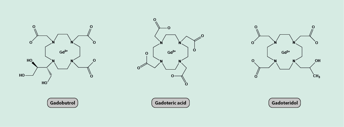
The most commonly used paramagnetic contrast agents for clinical MRI are complexes of Gd 3+ ions (these gadolinium ions have a large number of unpaired electrons and hence a large electron magnetic moment). The European Medicines Agency (EMA) in their 2017 review of gadolinium contrast agents advised that the gadolinium agents gadobutrol, gadoteric acid and gadoteridol (Figure 18) are safe for general intravenous use.
There is however debate over the safety of gadolinium-based MRI contrast agents. Recent studies indicate that small amounts of Gd3+ ions may be deposited and retained in a particular area of the brain. This may be a particular issue for individuals with insufficient kidney function, when the Gd3+ ions are not sufficiently rapidly excreted from the body. There is currently no evidence that such minor gadolinium deposition in the brain causes harm, but organisations such as EMA advised the restricted use of certain gadolinium-based agents which may be more likely to be retained by the body (such as gadodiamide, gadopentetic acid, and gadoversetamide).
The search for alternative paramagnetic substances to replace gadolinium-based agents is an area of ongoing research in clinical MRI. Alternatives include manganese ions, Mn2+. For example, manganese ions are contained in enzymes in pineapple and blueberry juices, making these potential contrast agents for oral use for some specific MRI applications. No sufficiently chemically stable synthetic Mn2+ substances for general use as contrast agents have so far been identified, but the search is ongoing. Another possibility are magnetic iron-containing nanoparticles. The body also supplies its own, endogenous contrast agent, in the form of haemoglobin molecules in blood. This paramagnetic Fe2+/ Fe3+ complex is exploited in functional MRI, fMRI, investigations (see below).
Catalogue of MRI experiments, and what they highlight / display
Below we give a brief summary of the most commonly used MRI experiments in clinical practice. Usually, a combination of different MRI experiments with or without exogenous contrast agents are used for a clinical investigation.
A useful characteristic of MRI experiments are the two experimental variables echo time (TE) and repetition time (TR):
- echo time (TE) is the time between the initial radiofrequency excitation pulse and the peak of the induced signal;
- repetition time (TR) is the time from the initial radiofrequency excitation pulse to the application of the next excitation pulse.
T1 weighted imaging (T1WI) is a basic pulse sequence used in MRI, in which the final image primarily demonstrates differences in the T1 relaxation times of different tissues. T1WI tends to have short TE and TR times. Longer TR times would mean that at the time point of measurement, all 1H magnetisation would have recovered alignment with the magnetic field B0, and thus there would be no T1-defined contrast. Very few structures naturally have a high signal intensity on a T1 weighted image, making T1WI useful when contrast agents are used, because tissues experiencing the most intense / efficient relaxation enhancement due to the contrast agent appear very bright on the image.
T2 weighted imaging (T2WI) primarily demonstrates differences in the T2 relaxation times of different tissues. In contrast to T1WI, T2WI requires longer TE and TR times. A characteristic of T2 weighted images is the high signal intensity of 1H spins in water molecules. This makes T2WI particularly useful in the examination of oedema, soft tissue tumours of all kinds, infarction, inflammation and infection.
Proton density weighted images (PDWI) examine the number of 1H spins in a voxel rather than their relaxation times. PDWI images result from T1 and T2 contrast being minimal. They have short TE times to minimise T2 effects, and long TR times to minimise T1 effects. PDWI yields excellent contrast between fluid and cartilage, making it ideal in the MRI examination of joints, such as the jaw joint.
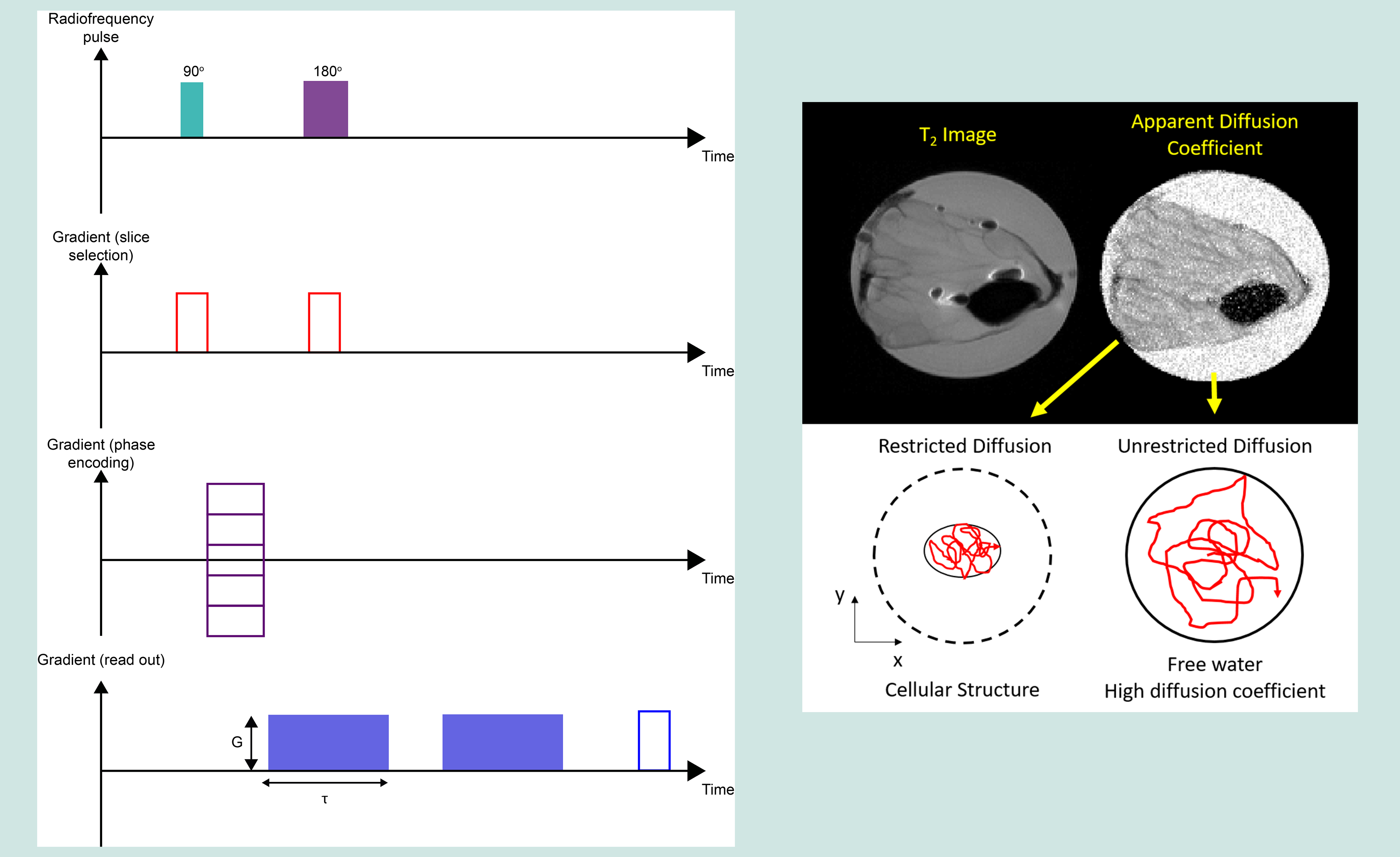
Diffusion-weighted imaging (DWI) is designed to detect the movement of water molecules. It is slightly different to T1WI and T2WI because it encodes whether within a voxel the water molecules undergo free diffusion, or if their movement over a specific time is constrained (for example inside a fibre-based structure). Water molecules diffuse relatively feely in the extracellular space, but their movement is significantly restricted in the intracellular space. The fundamental principle behind DWI is the attenuation of T2-signal, based on how easily water molecules are able to diffuse in a particular region / tissue. DWI is particularly useful in tumour characterisation (for example, in characterising the morphology of salivary glands), in investigations of damage of cranial nerves (because water diffusion in nerve tissue is extremely directional, along the nerve axons; see Figure 21), and in early identification of strokes. DWI also has a role in magnetic resonance angiography (MRA) because it enables the imaging of blood vessels without radioactive agents. A major issue with DWI is so-called ‘shine through’, an artefact where high T2-signal intensity from other structures is 'shining through' to the DWI image. Another important aspect for DWI are the mathematical models of diffusion of water molecules used to reconstruct images from this type of experiment.
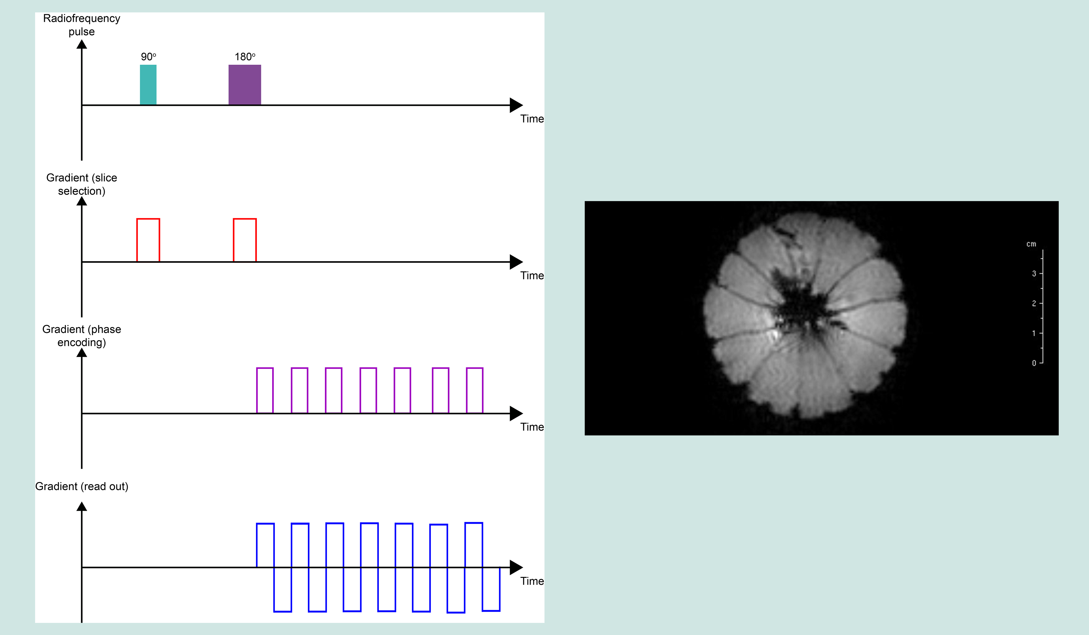
Echo planar imaging (EPI) experiments acquire multiple echoes of different phases, using rephasing gradients. This is accomplished by rapidly reversing the read-out or phase-encoding gradient. Echo planar sequences can use solely gradient echoes or may combine a spin echo with gradient echoes. EPI has a short imaging time: the whole image can be acquired within one TR period. EPI is one of the few ways to measure fMRI (see below) signals because it is so fast to acquire. The speed of data acquisition also results in decreased motion artefacts, but there are decreased spatial resolution and sensitivity to magnetic effects such as chemical shift artefacts, including 1H spins in water molecules precessing off resonance. This problem is typically resolved by using so-called fat-suppression techniques (the second largest pool of 1H in the body are fat molecules. Occasionally, these 1H resonances are used for imaging purposes, but more often these signals negatively interfere with imaging based on 1H in water molecules, so fat-based 1H resonances usually need to be suppressed in data acquisition). These artefacts result in geometric distortions of the final image. This effect is caused by magnetic field inhomogeneities and it particularly prominent in anatomic regions with an air-tissue interface (such as the oral cavity). For EPI to be useful and reliable, very high-resolution gradients have to be used.
Functional magnetic resonance imaging (fMRI) uses the paramagnetic properties of deoxyhaemoglobin in blood as an endogenous contrast agent. During activity, cells require more oxygen; this diffuses out of the capillaries and into the tissue leaving behind more deoxyhaemoglobin. Therefore, one would expect more local paramagnetism and faster relaxation of signal, and therefore less intense signal compared to areas containing oxygenated blood.
Applied to the brain this is a very powerful technique as oxygen use is highly localised to functional brain regions. There exists a counterintuitive phaenomenon though during brain activity and therefore enhanced oxygen usage: the brain sends messages to dilate the arteries and thus oversupplies the area with more oxygenated haemoglobin. This in essence reduces the relative local paramagnetism within the voxel and actually more signal is observed! Obviously, fMRI measurements require very careful interpretation.
Common maxillofacial MRI applications
MRI is the routine investigation for soft tissue pathology of the head and neck where detailed imaging is required. This includes salivary gland disease, planning for salivary gland surgery, the staging, treatment and detection of recurrence of oral and oropharyngeal cancers, some benign soft tissue conditions of the head and neck and some forms of temporomandibular joint disease. It may be supplemented with conventional X-ray based CT scans (for example of the thorax in cancer staging) or comparative images made (when for example, greater detail of possible bone invasion by cancer is needed prior to treatment planning). Although metallic implants have always formed a contraindication to MRI, modern MRI / pacemaker combinations are often safe. Most modern facial and dental implants are made from titanium (or ceramic materials) and thus are ‘safe’ in an MRI scanner, but can still distort MRI results considerably (because the magnetic susceptibility of these materials is different from that of bone or soft tissues). MRA, magnetic resonance angiography, is the standard pre-operative MRI investigation of the blood vessels (with contrast agent) of the distal (outer part) leg when planning to use a free fibula flap in head and neck reconstruction.
More recent developments in MRI
Real-time MRI / MRI videos
For a long time it was assumed that due to long scanning times, obtaining MRI videos (real-time MRI), depicting real-time events would only be possible with poor image quality. However, with new image-construction algorithms removing this constraint, real-time MRI is now a promising technique to study the dynamics of the airway, lips, tongue, soft palate and vocal folds during breathing, speaking or swallowing. Real-time MRI currently utilises the fast low angle shot (FLASH) sequence. FLASH is a gradient-echo sequence (see above) with a low flip angle combined with a very fast repetition time. This allows rapid repetition of the basic sequence, so when iterated allows real-time MRI videos to be produced. Current sequences have a temporal resolution of 20 to 30 ms, with acceptable spatial resolution (see an example on our page about swallowing). The method is on its way to clinical exploration and evaluation, but is not yet widely used in clinical practice. One can envisage real-time MRI to become useful for maxillofacial surgical planning, for long-term monitoring after major ablative and reconstructive surgery, as well as to provide better insight into the recovery of mechanical functionality (breathing, swallowing, speaking).
Hyperpolarisation
As discussed above, when a magnetic field is applied to a system of randomly orientated nuclear magnetic spins, only a small surplus aligns with the magnetic field. Hyperpolarisation is an NMR technique which attempts to increase the proportion of spins which on average will align with the magnetic field, so when a measurement is performed, higher signal intensities are recorded. Currently, the most common hyperpolarisation techniques in the laboratory are para-hydrogen induced polarisation (PHIP; which chemically incorporates polarised hydrogen gas into molecules) and dynamic nuclear polarisation (DNP; which physically transfers higher polarisation from electrons to nuclear spins). Similarly, optical pumping methods can produce highly polarised 129Xe gas (noble gas) which might become useful for functional imaging of the vocal cavities and lungs. Hyperpolarisation MRI techniques may also lift restrictions in general about which isotopes one could use for imaging, other than 1H. For example, small but physiologically important 13C-enriched molecules may then be able to provide unique insight into physiological and pathophysiological processes. Hyperpolarisation is a highly active research area in NMR spectroscopy and MRI (clinical and otherwise in materials science) but still a long way away from clinical practice. Hyperpolarised agents are exogeneous and must be injected or inhaled but have limited lifetimes as these agents are not in their equilibrium state and thus want to return to thermal equilibrium; this may happen too rapidly for useful NMR or MRI applications.
Localised spectroscopy
The basic idea is simple: suppose one can use some MRI techniques to specify and select a particular voxel in an object / tissue, followed by taking a NMR spectrum / fingerprint of the biochemistry / physiology in this particular voxel taking advantage of all the rich molecular information encoded in NMR spectra. The idea is clearly attractive, it promises real-time direct insight into the functioning of living tissue in a non-invasive way and at a molecular level of information, such as identifying metabolites (as is increasingly done in biochemistry investigations ex vivo, in samples such as urine samples). For example, it takes around 10 to 30 minutes to obtain 1H NMR spectra of most brain metabolites in one selected voxel. So metabolic mapping of larger areas is too time consuming for the time being.
For the time being (2019), there are ideas and laboratory experiments, exploring how these ideas could be realised. Some challenges are obvious from what we have discussed so far: a small voxel will only provide a very poor signal-to-noise ratio of a NMR spectrum taken over the small voxel (so, any major improvements in signal intensity will be crucial preconditions; this is one area where in the future hyperpolarisation (see above) might be useful). In terms of taking 1H NMR spectra of metabolites in a voxel, the high concentration of water (and lipids) in living tissues now is a disadvantage: if one wants to take 1H NMR spectra of metabolites in a voxel, one needs to be able to highly effectively suppress the 1H NMR signals of water and/or lipid molecules in order to detect the signatures of the much less abundant metabolite molecules (most MRI scanners are technically equipped for this). Being able to directly examine metabolism by localised 1H NMR spectroscopy looking at minority molecules would / will hugely increase the power of MRI methods in medicine in detecting and characterising diseases that are not well characterised by any of the properties of water (or lipid) molecules alone – as is exploited in traditional MRI methods. The methodologies for doing just that are in the early stages of development – but are sufficiently important to make it a fairly safe prediction that sooner or later combining the ‘best of both worlds’ from NMR spectroscopy and MRI will become a well-established reality in clinical practice.